|
The logistic function appears often in simple physical and probabilistic experiments. A normalized logistic is also known as an S-curve or sigmoid function. The first derivative of this function has a familiar bell-like shape, but it is not a Gaussian distribution. Many use a Gaussian to describe data when a logistic would be more appropriate. The tails of a logistic are exponential, whereas the tails of a Gaussian die off very quickly. To decide which distribution makes more sense, we must must be aware of the conceptual model for the underlying phenomena.
In biology, the logistic describes population growth in a bounded environment, such as bacteria in a petri dish. In business, a logistic describes the successful growth of market saturation. In engineering, the logistic describes the production of a finite resource such as an oilfield or a collection of oilfields.
After discussing examples, we will see how a bound to exponential growth leads to logistic behavior. There are other forms of the logistic function with extra variables that allow more arbitrary shifts and scaling. First, I limit myself to the form derived most naturally from the Verhulst equation. Normalizations clarify the behavior without any loss of generality. Finally, I use a change of variables for fitting recorded data in physical units.
Exponential (geometric) growth is a widely appreciated phenomenon for which we already have familiar mental models. Investments and populations grow exponentially (geometrically) when their rate of growth is proportional to their present size. You can take almost any example of exponential growth and turn it into logistic growth by putting a maximum limit on its size. Just make the rate of growth also proportional to the remaining room left for growth. Why is this such a natural assumption?
Let us consider the bacteria in a petri dish. This is an easy way to create a logistic curve in nature, and the mental model is a simple one.
A petri dish contains a finite amount of food and space. Into this dish we add a few microscopic bits of bacteria (or mold, if you prefer). Each bacterium lives for a certain amount of time, eats a certain amount of food during that time, and breeds a certain number of new bacteria. We can count the total number of bacteria that have lived and died so far, as a cumulative sum; or more easily, we can count the amount of food consumed so far. The two numbers should be directly proportional.
At the beginning these bacteria see an vast expanse of food, essentially unlimited given their current size. Their rate of growth is directly proportional to their current population, so we expect to see them begin with exponential growth. At some point, sooner or later, these bacteria will have grown to such a size that they have eaten half the food available. At this point clearly the rate of growth can no longer be exponential. In fact, the rate of consumption of food is now at its maximum possible rate. If half the food is gone, then the total cumulative population over time has also reached its halfway point. As many bacteria can be expected to live and die after this point as have gone before. Food is now the limiting factor, and not the size of the existing population. The rate of consumption of food and the population at any moment are in fact symmetric over time. Both decline and eventually approach zero exponentially, at the same rate at which they originally increased. After most of the food has disappeared, the population growth is directly proportional to the amount of remaining food. As there are fewer places for bacteria to find food, then fewer bacteria will survive and consume a lifetime of food. Although the population size is no longer a limit, their individual rates of reproduction still matter.
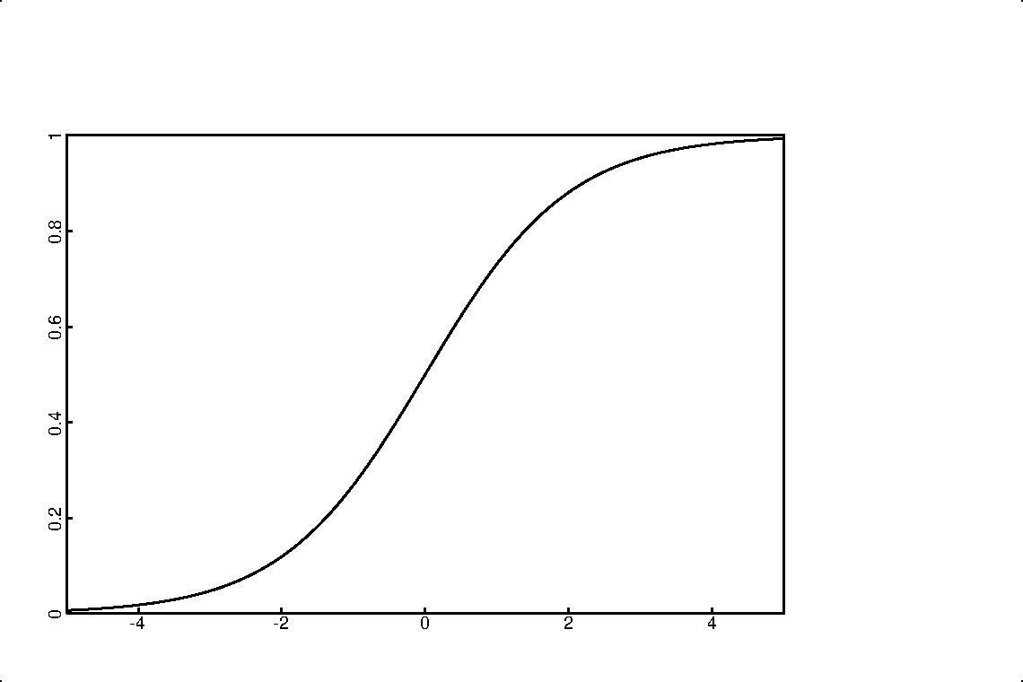
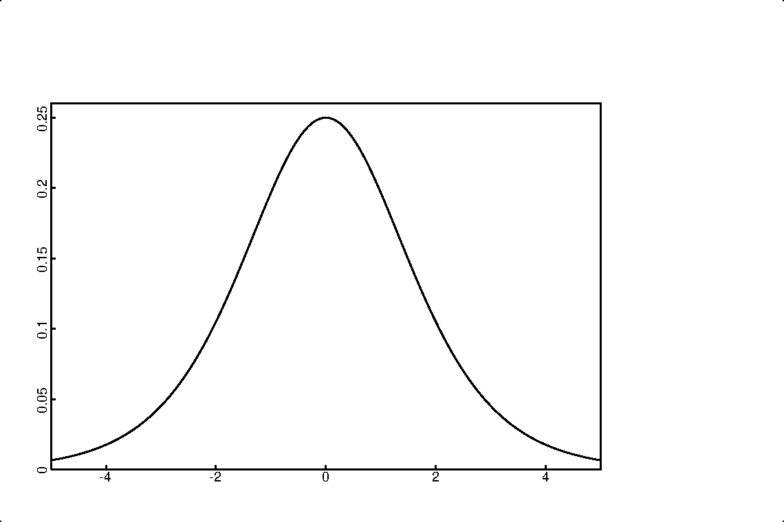
The logistic function can be used to describe either the fraction of the food consumed, or the accumulated population of bacteria that have lived and died. The first derivative of the logistic function describes the rate at which the food is being consumed, and also the living population of bacteria at any given moment. (If you have twice as many bacteria, then they are consuming food at twice the rate.) This derivative has an intuitive bell shape, up and down symmetrically, with exponential tails. The logistic is the integral of the bell shape: it rises exponentially from 0 at the beginning, grows steepest at the half-way point, then asymptotically approaches 1 (or 100%) at later times. The time scale is rather arbitrary. We can adjust the units of time or the rates of growth and fit different populations with the same curve.
Let us quickly examine two slightly messier examples, to see the analogies.
The market share of a given product can be expressed as a fraction, from 0% to 100%. All markets have a maximum size of some kind, at least the one imposed by a finite number of people with money. Let us assume someone begins with a superior product and that the relative quality of this product to its rivals does not change over time. The early days of this product on the market should experience exponential growth, for several reasons. The number of new people exposed to this new product depends on the number who already have it. The ability of a business to grow, advertise, and increase production is proportional to the current cash-flow. A exponential is an excellent default choice, in the absence of other special circumstances (which always exist).
Clearly, when you have a certain fraction of the market, geometric growth is no longer possible. Peter Norvig coined this as Norvig's Law: “Any technology that surpasses 50% penetration will never double again (in any number of months).” But let's also assume we have no regulatory limits and no one abusing a larger market share (bear with me). This product should still naturally tend to a saturated monopoly of the market. Such market saturation is typically drawn as a sigmoid much like a logistic. In fact it is a logistic, given no other mechanisms. After saturation, the rate of change of market share is proportional to the declining number of new customers. In any given month, a consistent fraction of the remaining unconverted customers will convert to the superior product. That is, we have a geometric or exponential decline in new customers for each reporting period.
Finally, let us examine the discovery and exhaustion of a physical resource, such as mining a mountain range, or exploration and production of oil in an field. The logistic has long been used to predict the production history, the number of barrels of oil produced a day, in any oil field. The curve also accurately handles a collection of oilfields, including all the oil fields in a given country. Such a calculation was first used by King Hubbert in 1957 to predict correctly the peak of total US oil production in the early 1970's.
Earliest oil production is easily exponential, like many business ventures. As long as there is vastly more oil to be produced than available, then previously produced oil can proportionally fund the exploration and production of new oil wells. Success also increases our understanding of an area and improves our ability to recognize and exploit new prospects, so long as there is no noticeable limit to those prospects. At some point though, the amount of oil in a given field becomes the limiting factor. Like bacteria in a petri dish, fewer oil wells find a viable spot in the oil field in order to produce a full lifetime. The maximum rate of production is achieved, very observably, when half of the oil has been produced that will ever been produced. (That is not to say that oil does not remain in the ground, but it cannot be produced economically, using less energy than obtained from the new oil.)
Oil production from individual oil fields do often show asymmetry, falling more rapidly or more gently after a peak than expected from the rise. Petroleum engineers have learned that deliberately slowing production increases the ultimate recoverable oil from a field. Gas production of a single field tends to maintain a more constant rate of production until the pressure abruptly fails, dropping production to nothing. But while individual fields may have unique production curves, collections of fields in a region or country tend to follow a more predictable logistic trend, with the expected symmetry.
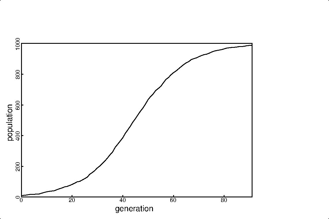
We can contrive a simple numerical game that should simulate such growth. We have a resource that can support a maximum population of 1000 creatures. We will begin by dropping 10 creatures into this resource. All are likely to find an unoccupied location. With every generation, each existing creature has a 10 percent chance of spawning a new creature. These new creatures drop again at random into one of the 1000 possible locations. If the location is not previously used, then the creature survives. If the location is already occupied, then the new creature dies. In early generations, 99 percent of the possible locations are still free, so each new creature will almost certainly survive. We expect early generations to show 10 percent geometric growth. As the population increases, however, available locations decrease and we see more collisions. By the time 500 of the available locations are filled, only half of each new generation will survive, dropping the rate of growth to about 5 percent. We will stop the game when 990 locations are full, when each new creature has only one percent chance of survival.
Here is a short Java program to simulate this population growth.
import java.util.Random;
import java.util.BitSet;
public class LogisticGrowth {
  public static void main(String...args) {
    Random random = new Random(1);
    int capacity = 1000;
    BitSet resource = new BitSet(capacity);
    for (int i=0; i< 10; ++i) { resource.set(i); }
    int population = 0, generation = 0;
    while ( (population=resource.cardinality()) < capacity-10) {
      System.out.println(generation+" "+population);
      for (int spawn=0; spawn<population; ++spawn) {
        if (random.nextInt(10) % 10 == 0 ) {
          resource.set(random.nextInt(capacity));
        }
      }
      ++generation;
    }
  }
}
The result of this simulation appears in figure 1.
Similarly, you can imagine bacteria spores landing in a petri dish at random. If food is available, a bacterium survives and breeds by launching new spores. If the food was already consumed by a prior bacterium, then the new one will die.
Bacteria probably do not fill a petri dish uniformly, but spread from a center. Most living populations will have some evolved ability to find food. Yet, such changes to the rules should only accelerate or decelerate growth, without changing the overall shape.
Similarly, marketing and oil exploration claim to do better than random selections. And skills are improved by past successes. Even so, the size of each new generation is still dominated by the size of the existing population and the absolute capacity of the resource.
The scenarios described above do not come close to representing all problems that can be modeled as a logistic curve. The function solves certain estimation problems involving the parameters of a Gaussian random variable. Such an S-curve is also convenient for signal processing applications such as neural networks. To help our intuition, I will nevertheless explain the notation with the previous examples in mind.
Keep in mind that these distributions also represent expectations or probabilities. Imagine that each limited resource is composed of a finite number of unique identities, such as an individual customer, a certain barrel of oil, a particular bit of food, or an empty spot on the dartboard. The logistic represents the probability that a unique quantum of a resource will be consumed by a particular moment in time. Since the same probability distribution applies to all quanta, you expect an actual realization to resemble a histogram with roughly the same shape. Thinking of the logistic as a probability distribution will help when we try fit actual data.
Let us use  to represent a fraction
of some quantity limited to values between 0 and 1.
This fraction is a function of time
to represent a fraction
of some quantity limited to values between 0 and 1.
This fraction is a function of time  .
.
We expect this fraction to increase over
time. The rate of increase, the first derivative,
will always be positive:
 |
Units of time are fairly arbitrary for such problems. For the function to approach a value of 1 asymptotically, time must continue to positive infinity. To avoid a small non-zero value to begin growth, we can allow the function to begin arbitrarily early at negative infinity, where it can approach 0.
The scale of time units, whether seconds or days, is also
arbitrary. We will choose a scale that most conveniently
measures a consistent change in the function.
Let us put the halfway point, at zero time so that
For earliest values of , we expect
to increase geometrically. That is,
we expect the rate of increase to be
proportional to the current value:
Similarly, as time increases and our
function approaches unity, we expect
the rate of growth to be proportional
to the remaining fractional capacity.
Let us combine these two proportions
(2) and (3) into
a single equation that respects both:
![$\displaystyle {d f(t) \over dt}\propto f(t) [1-f(t)] .$](img16.svg) |
The rate of growth at any time is proportional to the population and to the remaining available fraction. Both factors are always in play, though one factor dominates when the value of the function approaches either 0 or 1.
By centering this equation at zero time
with (1),
we can rearrange the Verhulst equation (4)
and integrate for  with
with
Some versions include include arbitrary scale factors for time or for the fraction itself. We have avoided those by normalization to fractions and convenient time units. Later we will use a change of variables useful for fitting physical data.
First notice that this equation is anti-symmetric,
with an additive constant:
![$\displaystyle 1- f(t) = 1/[ 1 + \exp(t)]$](img30.svg) |
 |
 |
|
 |
|
 |
(8) |
The derivative  is often a
more interesting quantity than itself.
For example, in oil production, this might be
the number of barrels produced a day (with an
appropriate scale factor). It could be the annual
growth in market share, the rate at
which a population grows, or the rate of
consumption of food.
is often a
more interesting quantity than itself.
For example, in oil production, this might be
the number of barrels produced a day (with an
appropriate scale factor). It could be the annual
growth in market share, the rate at
which a population grows, or the rate of
consumption of food.
In this form, the derivative (9) has unit area, integrating to 1. The equation is also useful as the probability distribution function (pdf) that a given resource (food, oil, or customer) will be used at a particular moment in time.
Assume you have some data that you think might be described by a logistic curve. You have the data up to a certain point in time. You might not be halfway yet. Can you see how well the data are described by a logistic? Can you predict the area under the curve, or the halfway point?
From a partial dataset, we do not yet know the ultimate true capacity, and we use real time units. Let us use another form of the Verhulst equation more useful for real-world measurements.
To get a form similar to that used by
Verhulst for his population model,
we replace
 |
(10) |
 for measurable time units,
with
for measurable time units,
with  for an unknown time scaling, and
with
for an unknown time scaling, and
with
 for an unknown reference time.
We also substitute
 |
(11) |
 is a measurable capacity
or population, and
is a measurable capacity
or population, and  is an unknown upper
limit, called the “carrying capacity.”
is an unknown upper
limit, called the “carrying capacity.”
The reference time
is when we expect
to reach half of the maximum capacity:
With these substitutions, we rewrite the
Verhulst equation (4) as
 , and
the vertical intercept of the line
is .
, and
the vertical intercept of the line
is .
The quantity on the left of equation (
 )
could be called the fractional rate of growth.
It is the current rate of growth divided by
the cumulative value so far. We do not need
to know ultimate rates, capacities, or
reference times to calculate this quantity.
At earliest times, when is small relative to ,
the fractional rate of growth (13) achieves a maximum
value of .
)
could be called the fractional rate of growth.
It is the current rate of growth divided by
the cumulative value so far. We do not need
to know ultimate rates, capacities, or
reference times to calculate this quantity.
At earliest times, when is small relative to ,
the fractional rate of growth (13) achieves a maximum
value of .
We can make a graph with this fractional rate of growth
on the vertical axis, and with the cumulative value
on the horizontal. For every time at which
we measure these two quantities, we can place a point
on the graph. All values are positive and fall
inside the upper-right quadrant.
If the data fit a logistic curve,
then we should be able to draw a straight line
through them. The slope and vertical intercept
of the line allow us to estimate the unknown constants
and . The vertical intercept, where
 ,
is the rate ,
and the horizontal intercept is the maximum carrying
capacity
,
is the rate ,
and the horizontal intercept is the maximum carrying
capacity
 .
.
So what about the reference time,
?
As time increases our data points move along this
line, but not uniformly. Time units do not appear
explicitly, except as a sampling parameter.
The time
corresponds to the data
point with half of the ultimate capacity, as in (12).
We may not have enough data to identify this point
from this graph.
Another drawback to this particular way of graphing data
is that early times will show much greater
scatter than later times. When
 and are small,
their ratio will show greater variation
for small variations in either. This particular
linearization is more suitable for an age of graph paper.
I prefer to fit the logistic more directly.
and are small,
their ratio will show greater variation
for small variations in either. This particular
linearization is more suitable for an age of graph paper.
I prefer to fit the logistic more directly.
Using the
definition (12) as a boundary condition,
we can also rewrite the logistic function (7)
in measurable units:
is the ultimate
maximum value of .
If we fit directly, our fit should improve with
time. The value is a cumulative one, integrating measurements
over longer periods of time. Again, we can expect more
variation at earlier times.
Instead, let us examine an absolute rate of increase  that we can also measure:
 .
.
Now we have a function with more consistent variations over time. The incremental change during a short interval of time will tend to follow the underlying distribution, with greater deviations as we shorten the interval.
Actually, it is not difficult simply to scan reasonable
values for all three parameters , , and
and minimize some misfit to .
You can also plot the misfit as contours of multiple parameters
and get a better idea of your sensitivity to each.
Choosing a best measure of misfit is still necessary.
Least-squares, the default choice for many, makes sense only
if you think that errors
in your measurements are Gaussian and consistent over time.
This seems unlikely. Lower magnitudes have less potential
for absolute variation than larger ones. We could instead
minimize errors in the ratio of a measured magnitude of
to the expected magnitude. Or equivalently,
we can minimize errors in the logarithm of .
If we minimize the square of those errors, then we
are assuming that variations in our measurements are multiplicative,
following a log Gaussian distribution. This is much
better, but I think still not optimum.
Another way to think of the problem is that the logistic
derivative in (16)
describes a probability of a particular quantity being exploited
or consumed at a particular point in time. A given customer,
bacterium, or barrel of oil, is most to appear near the peak
time
rather than near the tails. Given a certain realization
of that probability, our recorded data, what parameters maximize
the probability of that data? It turns out that this likelihood
is maximized by a minimum cross-entropy.
Let our recorded data be pairs of samples
 indexed by
  .
Then the best distribution should minimize
.
Then the best distribution should minimize
is a function of these three unknown parameters
 .
.
The that minimizes this cross-entropy is the one
that makes the actually recorded data most probable.
Because we have not necessarily sampled the entire function,
we should renormalize both and  over the range of available
  before evaluating.
Normalization effectively ignores the unknown capacity
and fits only the local shape of the curve.
The remaining two degrees of freedom and
can be exhaustively
searched with dense sampling. Once these are known, the best
can be calculated without normalization.
before evaluating.
Normalization effectively ignores the unknown capacity
and fits only the local shape of the curve.
The remaining two degrees of freedom and
can be exhaustively
searched with dense sampling. Once these are known, the best
can be calculated without normalization.
Neural networks and machine learning algorithms often use the same family of S curves for “logistic regression,” but motivate the equations differently.
Logistic regression attempts to estimate the probability of an event with a binary outcome, either true or false. The probability is expressed as a function of some “explanatory variable.” For example, what is the probability of a light bulb failing after a certain number of hours of use? Maybe more relevant, what is the probability a given drilling program will be economic, given some measurement of effort?
We start with a probability  of one outcome — say a successful well or a good lightbulb.
That leaves us with a probability of
of one outcome — say a successful well or a good lightbulb.
That leaves us with a probability of  for the alternative — a bad well, or a bad lightbulb.
Our explanatory variable
for the alternative — a bad well, or a bad lightbulb.
Our explanatory variable  could be a unit of time, as before, or some other factor.
We expect the probability
could be a unit of time, as before, or some other factor.
We expect the probability  either to increase or to decrease strictly as a function of .
Logistic regression uses the logit function, which is the logarithm
of the “odds.” The odds are the ratio of the chance of success to failure.
as .
The  function and the logistic function (7) are inverses
of each other.
function and the logistic function (7) are inverses
of each other.
Unlike our earlier derivation, we are not going to assume that our explanatory has been normalized and
shifted for our convenience, so we will use different symbols. Determining that scaling and shifting is
the work of logistic regression.
Logistic regression assumes that the function (5) is a linear
function of the explanatory variable .
 and
and  finds the appropriate horizontal scaling and the midpoint of our curve,
so that we could redefine a normalized
finds the appropriate horizontal scaling and the midpoint of our curve,
so that we could redefine a normalized
 and use our previous equations.
Fitting data with this curve (18) is still best addressed as a maximum likelihood optimization.
We have a record of successes and failures, each with different values of the
explanatory variable . We adjust the constants until the computed probability (18)
of these events is maximized.
Alternatively, we are fitting a straight line to a graph with a value of as the horizontal
abscissa and the logit function (18) as the vertical ordinate.
But a normal least-squares linear regression
will not distribute the errors as correctly as a maximum-likelihood optimization.
The log-odds might seem like an arbitrary quantity to fit, but it has a connection to information theory.
The entropy  of a single binary outcome with probability is defined as
 for the probability
  , which is
the most unpredictable distribution.
When the probability is low (near 0) or high (near 1), then the entropy approaches a minimum value of 0.
A lower entropy is a more predictable outcome, with 0 giving us complete certainty.
, which is
the most unpredictable distribution.
When the probability is low (near 0) or high (near 1), then the entropy approaches a minimum value of 0.
A lower entropy is a more predictable outcome, with 0 giving us complete certainty.
The derivative of the entropy with respect to gives us the negative of the logit function:
is a linear function of the variable then the
entropy is a second-order polynomial, with just enough degrees of freedom for a
single maximum and an adjustable width.


![$\displaystyle {d f(t) \over dt}= f(t) [1-f(t)] .$](img17.svg)
![$\displaystyle \left [ {1 \over f(t)} + {1 \over 1-f(t)} \right ] df(t)/dt$](img19.svg)

![$\displaystyle {d \over dt} \{ \log f(t) - \log [1-f(t)] \}$](img22.svg)
![$\displaystyle \log f(t) - \log [1-f(t)]$](img23.svg)

![$\displaystyle \log \left [ {f(t) \over 1-f(t)} \right ]$](img25.svg)


![$\displaystyle { \exp(-t) \over [ 1 + \exp(-t) ]^2 }
= {1 \over [ \exp(t/2) + \exp(-t/2) ]^2} ,$](img35.svg)


![$\displaystyle r [1-Q( {\tau} )/k] Q( {\tau} ) ;$](img47.svg)


![$\displaystyle Q( {\tau} ) = {k \over 1 + \exp[-r ( {\tau} - \bar{ {\tau} } )]} .$](img55.svg)
![$\displaystyle P( {\tau} ) \equiv
{d Q( {\tau} ) \over d {\tau} } =
{k r \over \...
... ( {\tau} - \bar{ {\tau} } )/2] + \exp[-r ( {\tau} - \bar{ {\tau} } )/2]\}^2} .$](img57.svg)
![$\displaystyle \min_{k, r, \bar{ {\tau} } } \sum_i \left \{ P^i ~ \log [ P^i ~/ ~ P( {\tau} ^i ) ]\right \} .$](img61.svg)

![$\displaystyle \log \left [ {p(x) \over 1-p(x)} \right ]$](img71.svg)


![$\displaystyle {d H(p) \over dp} = - \mbox{logit}(p).
% dH(p)/dp = -log(p) - 1 + log(1-p) + (1-p)/(1-p) = log[(1-p)/p] = -log[p/(1-p)]
$](img80.svg)