Notes on continuous wavelet transforms

William S. Harlan

Originally November 1996 – updated October 27, 2017

Introduction

First I will provide my own favorite definition of a continuous wavelet transform, which I wrote down in 1986 to rederive the results in Goupillaud et al [1]. (At the time, I was working down the hall from Pierre Goupillaud.) This continuous transform seemed much better suited to geophysical and acoustic applications than certain discrete transforms popular at the time, particularly Daubechies wavelets. Many wavelets have a broader spectrum than necessary, more suitable for compressing photographic images with sharp edges. A continuous transform can use simple Gaussian tapered monochromatic waves (one or multi-dimensional) which maximizes the locality in both time/space and frequency/wavenumber.

First, I will give the definition of what constitutes a valid “wavelet” for the transform. Second, the inverse of a wavelet transform will be derived to demonstrate why the transform works. Next, I will show how a wavelet-transform of a stretched function can be written as a simple function of the wavelet-transform of the original unstretched function. Such stretching is very useful in pseudo-spectral solutions of differential equations with spatially varying coefficients.

Next I dwell on the original Morlet wavelet, a Gaussian-tapered sinusoid, to show how resolution can be managed explicitly in both time and frequency domains.

(This is an expansion of a much older document [2] that stressed the application of wavelet transforms to seismic imaging. I have removed the geophysical details and have extended the discussion.)

Legal wavelets

I will closely imitate the continuous transform originally provided by Goupillaud, Grossman, and Morlet [1]. They provide forward and inverse transforms for related transforms, but without derivation.

Use the following Fourier convention to link a wavelet $w(t)$ and its Fourier transform $\tilde w (s)$:

$$\tilde w (s) = \int e^{-i 2 \pi s t } w(t) dt {\rm ~and}$$ (1)

$$w(t) = \int e^{i 2 \pi s t } \tilde w (s) ds .$$ (2)

(All integrals with unlabeled extremes are assumed to be over the entire real line.)

The following integral must exist for a wavelet to be suitable for a continuous transform over all frequencies.

  $$C_w = \int { 1 \over \vert s\vert } \tilde w (s) ds .$$ (3)

Thus, the spectrum of a valid wavelet must approach a zero value at zero frequency: $\tilde w (s) / \vert s\vert^\epsilon$ $\rightarrow 0$ as $s \rightarrow 0$ for some $\epsilon > 0$.

In fact many useful wavelets (such as the Morlet wavelet) will be non-zero at zero frequency and will not be valid for an infinite range of frequencies. Discrete transforms will prefer damped least-squares optimizations rather than simple integrals for transformations and will not require an analytic constant for normalization.

This wavelet need not correspond to any specific feature in our data. Rather, when convolved with data, the wavelet should suppress all but a band of frequencies. Because of the uncertainty principle, I must balance the narrowness of the bandwidth with the narrowness in time.

I recommend a Gaussian-tapered sinusoid, such as $w(t) = {\rm cos}(2\pi t) (e^{- \pi t^2 / c^2} )$. Such a wavelet is reasonably compact in both the time and frequency domain. (The constant $c$ adjusts the relative compactness, within the limits of the uncertainty principle.)

A valid wavelet can be used in an unfamiliar construction of a delta function.

  $$\int w(ut) du = C_w \cdot \delta (t) .$$ (4)

In effect, this integral says that many wavelets, stretched uniformly over all scales, will sum destructively everywhere but at $t=0$.

  $${\bf Proof:~} \int w(ut) du = \int \left \{ \int {1 \over \vert u\vert} \tilde w ( { s \over u } ) e^{i 2 \pi s t } ds \right \} du \ldots$$ (5)

Change variables from $(s,u)$ to $(s'=s,u'=s/u)$. The Jacobian is
$\partial (s,u) / \partial (s',u') = \vert s'/u'^2\vert$. Thus,

$$\int w(ut) du = \int \int \left \vert {u' \over s'} \right \vert \tilde w ( u' ) e^{i 2 \pi s' t } \left \vert { s' \over u'^2 } \right \vert ds' du'$$ (6)

$$= \int \int {1 \over \vert u'\vert} \tilde w ( u' ) e^{i 2 \pi s' t } ds' du'$$ (7)

$$= \left \{ \int {1 \over \vert u'\vert} \tilde w ( u' ) du' \right \} \cdot \left \{ \int e^{i 2 \pi s' t } ds' \right \}$$ (8)

$$= C_w \cdot \delta (t) .$$ (9)

Here, I use the familiar Fourier definition of a delta function, with the same restrictions.

The constraint of symmetry will also simplify the definition of a wavelet transform in the following section, but this assumption is optional:

  $$w(t) = w(-t) .$$ (10)

Forward and inverse transforms

Define a wavelet transform $F(u,a)$ of an $L^2$ function $f(t)$ by the following

  $$F(u,a) = \int w[u(a - t)] f(t) dt .$$ (11)

This transform decomposes the function as a function of position $a$ and local frequency $u$. When calculated discretely, the sampling need not be uniform over $a$ and $u$, but the weights should reflect the above integration.

Goupillaud et all [1] prefer $2^u$ or $u^{-1}$ instead of $u$ as the stretch factor. If you prefer an asymmetric wavelet, then you must use two transforms—the above, and the integral with the time-reversed wavelet.)

I find the following inverse, which simply scales and sums the transform with uniform weight over local frequency $u$:

  $$f(t) = C_w^{-1} \int F(u, a=t) du .$$ (12)

$${\bf Proof:~} C_w^{-1} \int F(u,a=t) du = C_w^{-1} \int \left \{ \int w[u(t - t' )] f(t') dt' \right \} du$$ (13)

$$= C_w^{-1} \int \left \{ \int w[u(t - t' )] du \right \} f(t') dt'$$ (14)

$$= C_w^{-1} \int C_w \delta(t-t') f(t') dt'$$ (15)

$$= f(t).$$ (16)

Here I make use of equation (4).

Most all these equations were implicit in Goupillaud et al [1], although I personally found it nontrivial to fill in the missing derivation of the results. I was also happy to stumble on equation (4), which continues to fascinate me.

Stretching

One application that frequently appears is a differential stretching of a function.

We will write

  $$g(\tau) = f[t(\tau)].$$ (17)

The stretching function $t(\tau)$ gives the input coordinate $t$ as a monotonically increasing function of the output coordinate $\tau$. Moreover, I will assume that the stretching function can be well approximated locally by a straight line.

$$t(\tau) \approx t(\tau_0 ) + (\tau - \tau_0 ) \cdot {dt \over d\tau} ( \tau_0 ) ~~~~{\rm and }$$ (18)

$$\tau(t) \approx \tau_0 + [ t - t (\tau_0 ) ] \cdot \left [ {dt \over d\tau} ( \tau_0 ) \right ]^{-1} .$$ (19)

Define forward and inverse wavelet transforms of $g(\tau)$ with the same wavelets as in definition (11) and inverse (12).

  $$G(v, b ) = \int w [ v ( b - \tau ) ] g (\tau) d\tau ~~~~ {\rm and}$$ (20)

  $$g(\tau) = C_w^{-1} \int G(v, b = \tau ) dv.$$ (21)

We would like to be able to express the transform $G(v, b)$ as a simple function of $F(u,a)$. The approximation (18) allows us to write

  $$G(v,b) \approx \left \vert {dt \over d\tau} ( b ) \right \vert^{... ...v \cdot \left [ {dt \over d\tau} ( b ) \right ]^{-1} , ~ a = t(b) \right \} .$$ (22)

We can perform an equivalent stretch on the transformed input by stretching the position $a$, and by scaling the local frequency $u$. Both operations require a simple two-dimensional mapping of the transformed function. The amplitude must be scaled as well.

$${\bf Proof: ~} G ( v, b) = \int w[v(b-\tau)] \cdot f[t(\tau)] d \tau$$ (23)

$$\approx \int w [ v(b-\tau)] \cdot f \left [ t(b) + (\tau-b) \cdot {dt \over d\tau} ( b ) \right ] d\tau \ldots$$ (24)

Substitute the variable of integration:

$$t' \equiv t(b) + (\tau-b) \cdot {dt \over d\tau} ( b ) ~~~~ {\rm and}$$ (25)

$$\tau = b + [ t' - t(b) ] \cdot \left [ {dt \over d\tau} ( b ) \right ]^{-1} .$$ (26)

Thus,

$$G ( v, b) = \int w \left \{ v \cdot [t(b) - t'] \cdot \left [ {dt \over d\tau... ...\} \cdot f(t') \cdot \left \vert {dt \over d\tau} ( b ) \right \vert^{-1} ~ dt'$$ (27)

$$= \left \vert {dt \over d\tau} ( b ) \right \vert^{-1} \int w \left... ...t \over d\tau} ( b ) \right ]^{-1} \cdot [t(b) - t'] \right \} \cdot f(t') d t'$$ (28)

$$= \left \vert {dt \over d\tau} ( b ) \right \vert^{-1} ~ F \left \{ u=v \cdot \left [ {dt \over d\tau} ( b ) \right ]^{-1} , ~ a = t(b) \right \} .$$ (29)

The symmetry of $w(t)$ was not necessary here.

Equation (22) is the result which allows us to perform the stretch directly on the wavelet-transformed function.

Morlet wavelets

A preferred standard wavelet is the Morlet wavelet [1], constructed from a symmetric cosine tapered by a Gaussian.

$$m(t) \equiv m_g(t) m_c(t) ,$$ (30)

$$\mbox{ where } m_g(t) \equiv e^{ - \pi (\bar{s}t / h )^2 }$$ (31)

$$\mbox{ and } m_c(t) \equiv \cos ( 2 \pi \bar{s}t) ,$$ (32)

$$\mbox{ so } m(t) = e^{ - \pi (\bar{s}t / h )^2 } \cos ( 2 \pi \bar{s}t) .$$ (33)

The constants $\bar{s}$ and $h$ do not vary during a wavelet transform. If we take the dimension $t$ as units of time in seconds, then $\bar{s}$ is the central frequency of the wavelet in hertz. The “half-width” $h$ controls the relative width of the taper in wavelengths.

The cosine has a base frequency of $\bar{s}$ and a wavelength of $1/\bar{s}$. The inclusion of a variable $\bar{s}$ for central frequency is just a convenience for managing units; $\bar{s}$ can be set to a constant without loss of generality. When we scan frequencies with a wavelet transform  (11), we can set $\bar{s}$ to 1 and substitute $u$ as frequency.

The envelope has a peak value of 1 at $t=0$ and drops to approximately half of this value at a separation of $h$ wavelengths.

$$m_g(0) = 1 ;$$ (34)

$$m_g[h/(2 \bar{s})] = m_g[-h/(2 \bar{s})]$$ (35)

$$= \exp (- \pi / 4) \approx 0.456 .$$ (36)

And so we call $h$ the half-width, in wavelengths, of the Gaussian taper.

The integral of the Gaussian envelope in time $t$ is

$$\int m_g(t) dt = \int e^{- \pi (\bar{s}t / h )^2 } dt = \frac{h}{\bar{s}} ,$$ (37)

equal to the half-width in units of time.

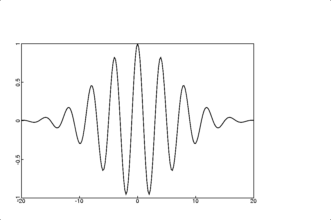
As an example, figure 1 shows one Morlet wavelet. We assume a time sampling interval of $1$ for a maximum Nyquist frequency of $0.5$. We choose a central frequency of $\bar {s}= 0.25$, and a halfwidth in wavelengths of $h=4$. We can see that one wavelength is $1/\bar{s}= 4$ time samples in length. The positive lobes at times of $t=\pm 8$ (third most positive values) are half the height of the peak. These half-strength peaks are separated by four wavelengths, as appropriate for $h=4$. The two peaks are also 16 time samples apart, as appropriate for four wavelengths of 4 samples each ( $h/\bar{s}= 4/0.25 = 16$).

Figure 1: Morlet wavelet with central frequency of $\bar {s}= 0.25$ and half-width $h=4$.

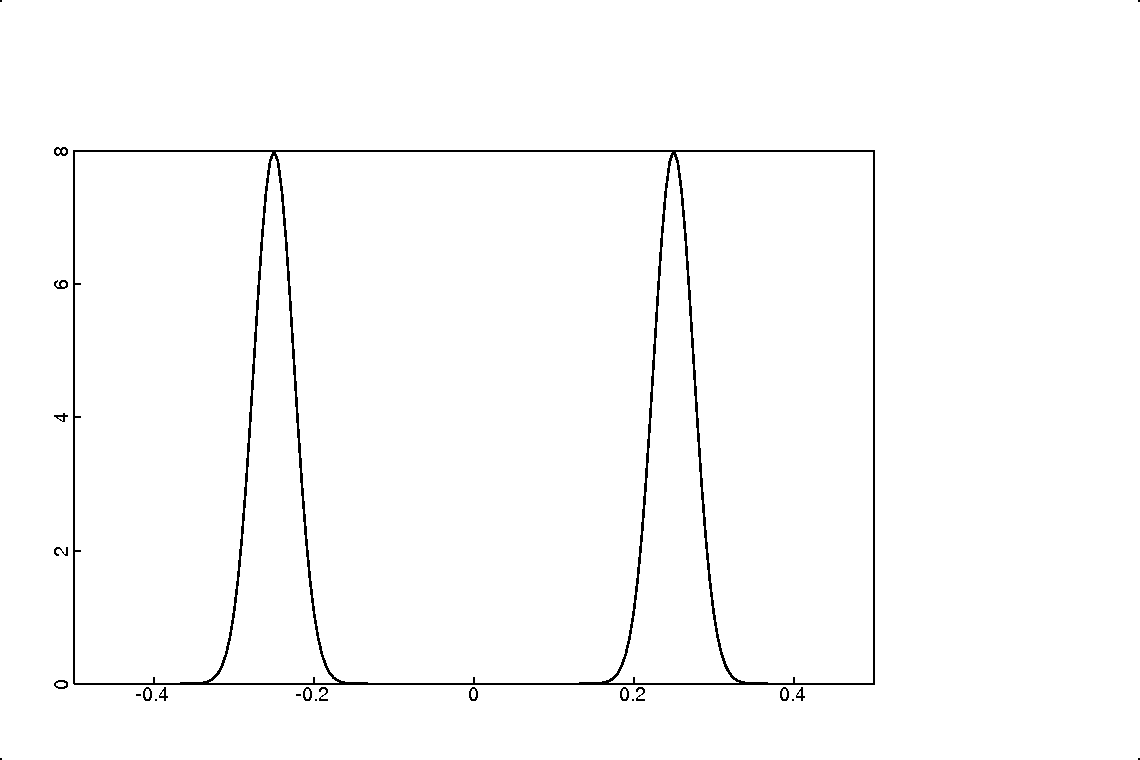
We can take the Fourier transform (1) of the Gaussian envelope as

$$\tilde m_g(s) \equiv \int e^{-i 2 \pi s t } m_g(t) dt = \int e^{-i 2 \pi s t } e^{ - \pi (\bar{s}t / h )^2 } dt$$ (38)

$$= \frac{h}{\bar{s}} e^{ - \pi ( h s /\bar{s})^2 } .$$ (39)

The equivalent half-width of this Gaussian is $\bar{s}/ h$, approximately spanning the range of values more than half of the peak value. This half-width $\bar{s}/ h$ in units of frequency is just the reciprocal of the half-width $h/\bar{s}$ in units of time.

Notice that the frequency half-width is directly proportional to the reference frequency $\bar{s}$. As we scan frequencies with a wavelet transform, we will see lower frequencies resolved with narrower ranges of frequencies. The resolution is constant in the log of frequency, which is why Morlet recommends sampling frequencies geometrically in octaves rather than linearly in frequency. When we construct a discrete basis of these wavelets for a discrete transform, there is no need to sample frequencies much more densely than this half-width.

The Fourier transform of the cosine is

$$\tilde m_c(s) \equiv \int e^{-i 2 \pi s t } m_c(t) dt = \int e^{-i 2 \pi s t } \cos (2 \pi \bar{s}t) dt$$ (40)

$$= \frac{1}{2}\delta (s+\bar{s}) + \frac{1}{2}\delta(s - \bar{s}).$$ (41)

The Fourier transform of the Morlet wavelet is the convolution of these two functions, for

$$\tilde m(s) \equiv \int e^{-i 2 \pi s t } m (t) dt = \int e^{-i 2 \pi s t } m_g (t) m_c (t) dt$$ (42)

$$= \tilde m_g(s) * \tilde m_c(s) = \int \tilde m_g(s') \tilde m_c(s -s') d s'$$ (43)

$$= \frac{h}{2 \bar{s}} e^{- \pi [ h ( s + \bar{s}) /\bar{s}] ^2 } + \frac{h}{2 \bar{s}} e^{- \pi [ h ( s - \bar{s}) /\bar{s}] ^2 }.$$ (44)

This gives us two Gaussians centered on the central frequency and mirrored on each side of zero.

Figure 2 shows the Fourier transform of the Morlet wavelet in figure 1, also with $\bar {s}= 0.25$ and $h=4$.

Figure 2: Fourier transform of Morlet wavelet in figure 1 with central frequency of $\bar {s}= 0.25$ and half-width $h=4$.

The resolution we care about is the narrowness of the spectrum about the central frequency $\bar{s}$. If we measure the standard deviation of one side of the Fourier transform (44), we are effectively measuring the width of the Fourier transformed envelope (39):

For quantifying resolution tradeoffs, a useful measure is the normalized second moment, or dispersion, in each domain. In time, the integral of the squared Gaussian taper is

$$\int \vert m_g(t) \vert^2 dt = \int e^{- 2 \pi (\bar{s}t / h )^2 } dt = \frac{1}{\sqrt{2}} \frac{h}{\bar{s}} ~,$$ (45)

and the second moment is

$$\int \vert m_g(t) \vert^2 t^2 dt = \int e^ { - 2 \pi (\bar{s}t / h )^2 } t^2 dt = \frac{1}{4 \sqrt{2} \pi}\frac{h^3}{\bar{s}^3} ~.$$ (46)

So the normalized second moment is

$$\Delta ^ 2 t = { \int \vert m_g(t) \vert^2 t^2 dt \over \int \vert m_g(t) \vert^2 dt } = \frac{1}{4 \pi} \frac{h^2}{\bar{s}^2} ;$$ (47)

$$\Delta t = \frac{1}{2 \sqrt{\pi}} \frac{h}{\bar{s}} ~.$$ (48)

Similarly we can measure second moments in the frequency domain.

$$\Delta ^ 2 s = {\int \vert \tilde m_g(s) \vert^2 s^2 ds \over \int \vert \tilde m_g(s) \vert^2 ds } = \frac{1}{4 \pi}\frac{\bar{s}^2}{h^2} ;$$ (49)

$$\Delta s = \frac{1}{2 \sqrt{\pi}}\frac{\bar{s}}{h} ~.$$ (50)

The uncertainty relation for resolution in time and frequency simplifies to

$$\Delta s \Delta t = \frac{1}{4 \pi}.$$ (51)

This inverse relationship is independent of both the half-width $h$ and the central frequency $\bar{s}$. The half-width in wavelengths $h$ controls the width of resolution in each domain, but cannot change this product of two widths. Improving the resolution in one domain necessarily reduces the resolution in the other. If we double the width of the envelope in the time domain, then we necessarily halve the width in the frequency domain.

References

1

P. Goupillaud, A. Grossman, and J. Morlet.
Cycle–octave and related transforms in seismic signal analysis.
Geoexploration, 23:85–102, 1984.

2

William S. Harlan.
Kirchhoff migration with one-dimensional wavelets.
This website: papers/wavelets.pdf, 1996.